Integrated multi-sensor navigation
Principal architecture of an integrated navigation system
Figure 1 illustrates principal architecture of a modern integrated navigation system. The system usually comprises of an inertial measurement unit (IMU), onboard computer, and external measurement systems (GNSS receiver, magnetometer, etc). The procedure of position, velocity, and orientation estimation is conventionally structured as follows. The onboard computer integrates navigation equations receiving the measurements of the specific force and angular rate from the IMU. However, accuracy of the navigation parameters determined by integrating the navigation equations degrades continuously due to IMU's instrumental errors, initial state errors, and the errors of numerical integration. That is why in parallel to integration the onboard computer estimates errors of the navigation parameters using information from external measurement systems. The obtained error estimates are further used to correct the position, velocity, and orientation information. In general, external measurements are not required to be available continuously, because the system is able to do dead reckoning using IMU information only. The rate of accuracy degradation during dead reckoning strongly depends on IMU accuracy class and quality of the "in-operation" calibration.
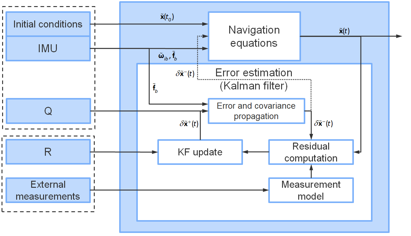
Fig. 1: Principal architecture of an integrated navigation system
Mathematical foundations of an integrated navigation system
Navigation equations
Navigation equations are the first order ordinary differential equations that describe motion of a point mass in the neighborhood of the Earth. The navigation equations, mechanized in the ECEF and the NED coordinate frames are given on the page dedicated to Inertial Navigation.
Navigation error propagation equations
Navigation error propagation equations are the equations that describe dynamics of the error of the navigation state. The errors are usually assumed to be small, which is why their dynamics can approximately be considered linear.
Errors of an INS mechanized in the ECEF frame are subject to
\begin{eqnarray}
\label{eq:ECEFerrorPropEq}
\delta \dot{\mathbf{x}}_e &=& \delta \mathbf{v}_e \\ \nonumber
\delta \dot{\mathbf{v}}_e &=& \left. \frac{\partial \mathbf{g}_e (\mathbf{x}_e)}{\partial \mathbf{x}_e^\mathrm{T}} \right|_{\tilde{\mathbf{x}}_e} \cdot \delta \mathbf{x}_e - 2 \pmb{\omega}_{ie} \times \delta \mathbf{v}_e - \left( \mathbf{R}_{\tilde{e}b} \tilde{\mathbf{f}}_b \right) \times \pmb{\psi}_{e \tilde{e}} + \mathbf{R}_{\tilde{e}b} \cdot \delta \mathbf{f}_b \\ \nonumber
\dot{\pmb{\psi}}_{e \tilde{e}} &=& -\pmb{\omega}_{ie} \times \pmb{\psi}_{e \tilde{e}} + \mathbf{R}_{\tilde{e}b} \cdot \delta\pmb{\omega}_{ib}
\end{eqnarray}
The system (\ref{eq:ECEFerrorPropEq}) can be obtained linearizing the ECEF navigation equations given on the Inertial Navigation page. The tilde symbol over a variable here and further on denotes an approximated/estimated value. By definition
\begin{eqnarray}
\label{eq:ECEFerrorDef}
\delta \mathbf{x}_e &=& \mathbf{x}_e -\tilde{\mathbf{x}}_e \\ \nonumber
\delta \mathbf{v}_e &=& \mathbf{v}_e -\tilde{\mathbf{v}}_e \\ \nonumber
\delta \mathbf{f}_b &=& \mathbf{f}_b -\tilde{\mathbf{f}}_b \\ \nonumber
\delta \pmb{\omega}_{ib} &=& \pmb{\omega}_{ib} -\tilde{\pmb{\omega}}_{ib} \\ \nonumber
\end{eqnarray}
\( \pmb{\psi}_{e \tilde{e}} \) is the orientation error vector introduced as follows:
\begin{equation}
\label{eq:PsiEcefDef}
\mathbf{R}_{eb} = \mathbf{R}_{e \tilde{e}} \mathbf{R}_{\tilde{e}b} \approx \left( \mathbf{I} + [\pmb{\psi}_{e \tilde{e}} \times] \right) \mathbf{R}_{\tilde{e}b}
\end{equation}
For an arbitrary vector \( \mathbf{a} = (a_1 \; a_2 \; a_3)^\mathrm{T} \)
$$
[\mathbf{a} \times] \overset{\mathrm{def}}{=}
\begin{pmatrix}
0 & -a_3 & a_2 \\
a_3 & 0 & -a_1 \\
-a_2 & a_1 & 0
\end{pmatrix}
$$
Errors of an INS mechanized in the NED frame are subject to the following dynamic system.
\begin{eqnarray}
\label{eq:NEDerrorPropEq}
\delta \dot{\pmb{\lambda}} &=& \left. \frac{\partial \mathbf{D}^{-1}(\pmb{\lambda}) \cdot \mathbf{v}_n}{ \partial \pmb{\lambda}^\mathrm{T}} \right|_{\tilde{\pmb{\lambda}},\tilde{\mathbf{v}}_n} \cdot \delta \pmb{\lambda} + \mathbf{D}^{-1}(\tilde{\pmb{\lambda}}) \cdot \delta \mathbf{v}_n \\ \nonumber
\delta \dot{\mathbf{v}}_n &=& \mathbf{A}_{21} \cdot \delta \pmb{\lambda} + \mathbf{A}_{22} \cdot \delta \mathbf{v}_n - \left( \mathbf{R}_{\tilde{n}b} \tilde{\mathbf{f}_b} \right) \times \pmb{\psi}_{n \tilde{n}} + \mathbf{R}_{\tilde{n}b} \cdot \delta \mathbf{f}_b \\ \nonumber
\dot{\pmb{\psi}}_{n \tilde{n}} &=& \left. \frac{\partial \pmb{\omega}_{in}(\pmb{\lambda}, \mathbf{v}_n)}{\partial \pmb{\lambda}^\mathrm{T}} \right|_{\tilde{\pmb{\lambda}},\tilde{\mathbf{v}}_n} \cdot \delta \pmb{\lambda} - \left. \frac{\partial \pmb{\omega}_{in}(\pmb{\lambda}, \mathbf{v}_n)}{\partial \mathbf{v}^\mathrm{T}_n} \right|_{\tilde{\pmb{\lambda}},\tilde{\mathbf{v}}_n} \cdot \delta \mathbf{v}_n - \pmb{\omega}_{in}(\tilde{\pmb{\lambda}}, \tilde{\mathbf{v}}_n) \times \pmb{\psi}_{n \tilde{n}} + \mathbf{R}_{\tilde{n}b} \cdot \delta \pmb{\omega}_{ib}
\end{eqnarray}
The system (\ref{eq:NEDerrorPropEq}) can be obtained linearizing the NED navigation equations given on the Inertial Navigation page.
The errors are defined as
\begin{eqnarray}
\label{eq:NEDerrorDef}
\delta \pmb{\lambda} &=& \pmb{\lambda} -\tilde{\pmb{\lambda}} \\ \nonumber
\delta \mathbf{v}_n &=& \mathbf{v}_n -\tilde{\mathbf{v}}_n \\ \nonumber
\mathbf{R}_{nb} &=& \mathbf{R}_{n \tilde{n}} \mathbf{R}_{\tilde{n}b} \approx \left( \mathbf{I} + [\pmb{\psi}_{n \tilde{n}} \times] \right) \mathbf{R}_{\tilde{n}b}
\end{eqnarray}
The \( 3 \times 3 \) matrices \( \mathbf{A}_{21} \) and \( \mathbf{A}_{22} \) take the following form
\begin{eqnarray*}
\mathbf{A}_{21} &=& \left. \frac{\partial \mathbf{g}_n (\pmb{\lambda})}{\partial \pmb{\lambda}^\mathrm{T}} \right|_{\tilde{\pmb{\lambda}}} - \left. \frac{\partial \left( 2 \mathbf{R}_{ne}(\pmb{\lambda}) \pmb{\Omega}_{ie} \mathbf{R}^{\mathrm{T}}_{ne}(\pmb{\lambda}) + \pmb{\Omega}_{en} \cdot \mathbf{v}_n \right) }{\partial \pmb{\lambda}^\mathrm{T}} \right|_{\tilde{\pmb{\lambda}}, \tilde{\mathbf{v}}_n} \\ \nonumber
\mathbf{A}_{22} &=& - \left. \frac{\partial \left( 2 \mathbf{R}_{ne}(\pmb{\lambda}) \pmb{\Omega}_{ie} \mathbf{R}^{\mathrm{T}}_{ne}(\pmb{\lambda}) + \pmb{\Omega}_{en} \cdot \mathbf{v}_n \right) }{\partial \mathbf{v}^\mathrm{T}_{n}} \right|_{\tilde{\pmb{\lambda}}, \tilde{\mathbf{v}}_n}
\end{eqnarray*}
The NED error propagation equations (\ref{eq:NEDerrorPropEq}) are usually evaluated assuming
$$ N(\phi) \approx R(\phi), \; M(\phi) \approx R(\phi), $$
where \( R(\phi) = \sqrt{M(\phi) N(\phi)} \) is the Earth's Gaussian mean curvature radius. The derivatives of \( R(\phi) \) with respect to \( \phi \) are neglected and the quantity \( R(\tilde{\phi}) \) is treated as a constant.
Measurement equations
A measurement equation is an equation that gives a relation between error-free aiding information \( \mathbf{y} \) and a navigation state vector \( \mathbf{z} \). In general the measurement equation can be written in the form
$$ \mathbf{y} = \mathbf{h} (\mathbf{z}). $$
However, real measurements \( \tilde{\mathbf{y}} \) always contain instrumental errors and thus present a superposition of the true value and an error. Therefore, formally,
$$ \tilde{\mathbf{y}} = \mathbf{y} - \delta \mathbf{y} = \mathbf{h}(\mathbf{z}) - \delta \mathbf{y}. $$
An equation of the form
\begin{equation}
\label{eq:GeneralMeasEq}
\Delta \mathbf{y} = \frac{\partial \mathbf{h} (\mathbf{z})}{\partial \mathbf{z}^\mathrm{T}} \cdot \delta \mathbf{z} - \delta \mathbf{y} \approx \tilde{\mathbf{y}} - \mathbf{h}(\tilde{\mathbf{z}}) + h.o.t.
\end{equation}
is called linearized measurement equation. The measurement error \( \delta \mathbf{y} \) is often composed both of deterministic and stochastic parts. Deterministic measurement errors are usually included into the navigation error state vector and are estimated by the navigation filter.
Discretization of linear systems
Consider linear system
\begin{equation}
\label{eq:LinearSysContinuous}
\dot{\mathbf{z}}(t) = \mathbf{A}(t) \mathbf{z}(t) + \pmb{\Gamma}(t) \mathbf{q}(t).
\end{equation}
Herein it is assumed that \( \mathbf{q}(t) \) presents zero-mean Gaussian white noise, i. e.
$$ \mathrm{E} \left[ \mathbf{q}(t) \right] = \mathbf{0}, \; \mathrm{E} \left[ \mathbf{q}(t) \mathbf{q}^\mathrm{T}(t) \right] = \mathbf{Q}(t) \delta(t - \tau). $$
The continuous system (\ref{eq:LinearSysContinuous}) is equavalent to discrete system
\begin{equation}
\label{eq:LinearSysDiscrete}
\mathbf{z}_{k+1} = \pmb{\Phi}_{k+1,k} \mathbf{z}_{k} + \mathbf{q}^{\ast}_{k},
\end{equation}
where \( \mathbf{z}_{k} = \mathbf{z}(t_{k}) \), \( \pmb{\Phi}_{k+1,k} = \pmb{\Phi}(t_{k+1}, t_{k}) \) is the transition matrix of the system (\ref{eq:LinearSysContinuous}), and
\begin{equation}
\label{eq:NoiseDiscrete}
\mathbf{q}^{\ast}_{k} = \int\limits_{t_{k}}^{t_{k+1}} \pmb{\Phi}(t_{k+1}, \tau) \pmb{\Gamma}(\tau)\mathbf{q}(\tau) d\tau.
\end{equation}
By definition, the transition matrix is the unique solution of the system
$$ \frac{d \pmb{\Phi}(t, t_{0})}{dt} = \mathbf{A}(t) \pmb{\Phi}(t, t_{0}), \; \pmb{\Phi}(t_{0}, t_{0}) = \mathbf{I}. $$
It is possible to show that the sequence \( \mathbf{q}^{\ast}_{k} \), defined by (\ref{eq:NoiseDiscrete}), presents discrete zero-mean Gaussian white noise, whose covariance matrix takes the form
\begin{equation}
\label{eq:DiscreteNoiseCov}
\mathrm{E} \left[ \mathbf{q}^{\ast}_{k} ( \mathbf{q}^{\ast}_{l})^\mathrm{T} \right] = \mathbf{Q}^\ast_{k} \cdot \delta_{kl} = \int\limits_{t_{k}}^{t_{k+1}} \pmb{\Phi}(t_{k+1}, \tau) \pmb{\Gamma}(\tau) \mathbf{Q}(\tau) \pmb{\Gamma}^\mathrm{T}(\tau) \pmb{\Phi}^\mathrm{T}(t_{k+1}, \tau) d\tau \cdot \delta_{kl}.
\end{equation}
The integral in (\ref{eq:DiscreteNoiseCov}) is commonly approximated as
$$ \mathbf{Q}^\ast_{k} \approx \pmb{\Gamma}(t_{k}) \mathbf{Q}(t_{k}) \pmb{\Gamma}^\mathrm{T}(t_{k}) \cdot (t_{k+1} - t_{k}). $$
Kalman filter
Dynamics of navigation system errors can be approximately considered linear as long as sensor errors, numerical errors, and errors of the initial condition are relatively small. From theory of stochastic processes it is known that the conditional expectation \( \mathrm{E[X|Y]} \) is the best estimate of the random variable \( X \) given the measurement \( Y = f(X) \). "The best" is understood in a sense that it minimizes the mean squared error. When dynamic system is linear and all the noises in it are white and Gaussian, the conditional expectation also appears to be normally distributed and thus is completely defined by its mean value and covariance matrix. The recursive formulae, describing evolution of the mean and covariance of the conditional expectation in linear case are commonly called Kalman filter.
Consider the discrete system
\begin{eqnarray}
\label{eq:SysKF}
\mathbf{z}_{k+1} &=& \pmb{\Phi}_{k+1,k} \mathbf{z}_{k} + \mathbf{q}_{k}, \\ \nonumber
\mathbf{y}_{k} &=& \mathbf{H}_{k} \mathbf{z}_{k} + \mathbf{r}_{k},
\end{eqnarray}
and assume that
\begin{eqnarray}
\label{eq:AssumptionsKF}
&&\mathbf{q}_{k} \sim N(\mathbf{0},\mathbf{Q}_{k}), \; \mathrm{E} \left[ \mathbf{q}_{k} \mathbf{q}^\mathrm{T}_{l} \right] = \mathbf{0}, \; k \ne l, \\ \nonumber
&&\mathbf{r}_{k} \sim N(\mathbf{0},\mathbf{R}_{k}), \; \mathrm{E} \left[ \mathbf{r}_{k} \mathbf{r}^\mathrm{T}_{l} \right] = \mathbf{0}, \; k \ne l, \\ \nonumber
&&\mathrm{E} \left[ \mathbf{z}_{k} \mathbf{r}^\mathrm{T}_{l} \right] = \mathbf{0}, \\ \nonumber
&&\mathrm{E} \left[ \mathbf{z}_{0} \right] = \hat{\mathbf{z}}_{0}, \; \mathrm{E} \left[ \left( \mathbf{z}_{0} - \mathrm{E} \left[ \mathbf{z}_{0} \right] \right) \left( \mathbf{z}_{0} - \mathrm{E} \left[ \mathbf{z}_{0} \right] \right)^\mathrm{T} \right] = \mathbf{P}_{0}.
\end{eqnarray}
Then the mean \( \tilde{\mathbf{z}}_{k}^{+} \) and the covariance matrix \( \mathbf{P}_{k}^{+} \) of the conditional expectation of the vector \( \mathbf{z}_{k} \) are subject to
\begin{eqnarray}
\label{eq:KF}
\tilde{\mathbf{z}}_{k+1}^{-} &=& \pmb{\Phi}_{k+1,k} \tilde{\mathbf{z}}_{k}^{+}, \\ \nonumber
\mathbf{P}_{k+1}^{-} &=& \pmb{\Phi}_{k+1,k} \mathbf{P}_{k}^{+} \pmb{\Phi}_{k+1,k}^\mathrm{T} + \mathbf{Q}_{k}, \\ \nonumber
\\ \nonumber
\mathbf{K}_{k+1} &=& \mathbf{P}_{k+1}^{-} \mathbf{H}_{k+1}^\mathrm{T} \left( \mathbf{H}_{k+1} \mathbf{P}_{k+1}^{-} \mathbf{H}_{k+1}^\mathrm{T} + \mathbf{R}_{k+1} \right)^{-1}, \\ \nonumber
\tilde{\mathbf{z}}_{k+1}^{+} &=& \tilde{\mathbf{z}}_{k+1}^{-} + \mathbf{K}_{k+1} \left( \mathbf{y}_{k+1} - \mathbf{H}_{k+1} \tilde{\mathbf{z}}_{k+1}^{-} \right), \\ \nonumber
\mathbf{P}_{k+1}^{+} &=& \left( \mathbf{I} - \mathbf{K}_{k+1} \mathbf{H}_{k+1} \right) \mathbf{P}_{k+1}^{-}.
\end{eqnarray}
Conventional types of integrated navigation systems
Traditional AHRS
Attitude and heading reference system is an equipment that provides a pilot or an autopilot with information on vehicle's orientation relative to Earth. Nowadays high-end AHRSs use precision inertial sensors and thus do not require aiding in order to provide highly accurate orientation information. However, such systems can hardly be used in many modern applications due to tough size, weight, and cost limitations. That is why engineers are very often forced to use low-cost miniature inertial sensors, whose relatively large instrumental errors cause the estimates of orientation angles to drift away from their true values very fast. In order to overcome drifts of roll and pitch estimates accelerometers can be used to determine attitude during unaccelerated motion. Heading drift, in turn, can be compensated by aiding using a magnetometer. This approach may be very attractive for some applications, because just a minimal set of onboard sensors is required and sensor fusion algorithms are relatively simple. However, accuracy degrades considerably during long intervals of dynamic flight, because correcting roll and pitch angles becomes impossible. For more details on implementation of such a system the reader can refer to the reference [1].
Integrated INS/GNSS
GNSS aided INS is nowadays the most widespread type of integrated navigation systems. Like INS it can provide smooth position, velocity, and orientation outputs at a high rate, but the errors do not drift away as long as sufficient number of satellite signals is available. Moreover, fusing measurements of IMU and GNSS allows to improve calibration of inertial sensors, which decreases considerably error growth rate in purely inertial mode during GNSS signal outages. There are three conventional levels of INS/GNSS integration:
- Loosely-coupled
- Tightly-coupled
- Deeply-coupled
In a loosely-coupled design GNSS equipment determines at first position and velocity of a vehicle based on satellite signals only. Afterwords this information is used to correct navigation parameters predicted by an INS.
Tightly-coupled systems do not compute intermediate values of the vehicle's position and velocity. Instead of it pseudoranges and range-rates are directly used as measurements in the navigation filter. The latter approach is more powerful because the INS can still be corrected when less than four satellites are visible.
Deeply-coupled design supposes combining satellite signal tracking and navigating into single process. This allows to improve robustness at highly dynamic motion and increases performance in environments with low signal-to-noise ratio.
Nowadays tightly-coupled design is considered state-of-the-art. Deeply-coupled systems have certain benefits, but are not yet widespread due to complexity of sensor fusion.
Air-data aided AHRS
Air data system (ADS) is an onboard electronic system that measures parameters of the outside airflow. Modern ADSs usually allow to measure outside air temperature (OAT), static pressure, stagnation pressure, angle of attack (AOA) and angle of sideslip (AOS). This information can further be used to derive the altitude of the aircraft and its speed relative to air. In air data aided mode an INS can provide accurate information on vertical speed, pressure level, and attitude both at low and high dynamics. However, heading remains unobservable and its drift cannot be compensated. In order to stabilize the error of heading it is additionally required to aid the INS by a three-axis magnetometer. More information on integration of INS with ADS and magnetometer can be found in the work [4].
Advanced topics
- IMU error models, Allan variance
- Shaping filters for colored noises, navigation state augmentation
- Generating input data for simulation
- Observability
- Integrity monitoring, fault detection and isolation
- Covariance matrix factorization
- Derivation of measurement equations
- Implementation, testing, and much more...
To learn more about the advanced topics, please contact us!
Recommended literature
- Farrell, J.A., Aided Navigation, GPS with High Rate Sensors, McGraw-Hill, USA, 2008.
- Groves, P.D., Principles of GNSS, Inertial, and Multisensor Integrated Navigation Systems, 2 ed, Artech House, Boston, 2013.