Inertial navigation
Inertial sensors
Accelerometers and gyroscopes are usually called inertial sensors. An accelerometer is a sensor that measures one or more projections of a specific force acting on a body. A gyroscope is a device for measuring projections of an angular rate of the body relative to some inertial coordinate frame. Nowadays the abovementioned sensors are usually rigidly attached to the moving object which is why the measured values present the projections onto a body-fixed coordinate frame. Inertial sensors can be classified into two groups according to their output type: non integrating and integrating.
Non integrating inertial sensors output the measured specific force and angular rate directly, while integrating sensors provide the user with the measurements of increments of velocity and orientation. Ring laser gyroscopes (RLG) and fiber optic gyroscopes (FOG) are integrating, because they employ Sagnac effect and thus their raw output presents angular increment. Microelectromechanical (MEMS) sensors are non integrating by their physical principles. However, some MEMS systems may sample measurements at a very high frequency and provide the user with numerically integrated signal at a much lower frequency.
Principles of inertial navigation
The core idea of inertial navigation consists in determining position and orientaion of a moving object by means of integrating numerically differential equations of motion of a point mass in the neighborhood of Earth. Angular rate and specific force present inputs to the dynamic system and need to be measured by onboard inertial sensors. Additionally, initial position, velocity, and orientation are required to be known.
Due to instrumental errors of inertial sensors, errors of numerical integration, model errors and the errors of the initial condition, the navigation information, computed by an inertial navigation system (INS), loses accuracy with time. Modern aerospace navigation systems that make use of well-calibrated RLGs and high-precision qaurtz accelerometers can provide a user with position information whose accuracy degrades at a rate of 1 nautical mile per hour. Consumer grade inertial sensors can hardly be used for positioning, because error growth rate appears too large.
Coordinate frames
Quasi-inertial coordinate frame
The origin \( P_i \) of the quasi-inertial coordinate frame (i-frame) is located in the Earth’s center of mass. The first axis \( \mathbf{i}_1 \) points towards the point of intersection at time \( t_0 \) of the zero meridian and the equatorial plane. The third axis \( \mathbf{i}_3 \) points from the origin towards the IERS reference pole. The second axis \( \mathbf{i}_2 \) is the orthogonal completion of \( \mathbf{i}_1 \) and \( \mathbf{i}_3 \) to a right-handed axes system.
Earth-centered Earth-fixed coordinate frame
ECEF frame (e-frame) is a coordinate system with the origin \( P_e \) in the Earth’s center of mass. The third axis \( \mathbf{e}_3 \) is pointing from the origin towards the IERS reference pole. The first axis \( \mathbf{e}_1 \) points from the origin towards intersection of the IERS reference meridian and the plane passing though the origin and perpendicular to \( \mathbf{e}_3 \). The second axis \( \mathbf{e}_2 \) completes the right-handed system.
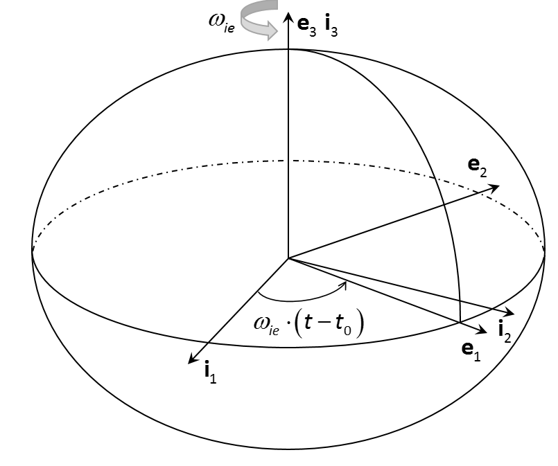
Fig. 1: i- and e-frames
Body-fixed coordinate frame
The origin \( P_b \) of the body-fixed coordinate frame (b-frame) is located in the arbitrarily chosen point of a vehicle. The first axis \( \mathbf{b}_1 \) points to front, the second axis \( \mathbf{b}_2 \) points right, and the third axis \( \mathbf{b}_3 \) completes the orthogonal right-handed system.
Local-level North-indicating coordinate frame
The third axis \( \mathbf{n}_3 \) of the Local-level North-indicating frame (n-frame) is perpendicular to the local tangent plane to WGS84 Ellipsoid. The first axis \( \mathbf{n}_1 \) is parallel to the North direction in the local tangent plane to WGS84 Ellipsoid. The second axis \( \mathbf{n}_2 \) completes the right-handed system. Origin of the n-frame can be chosen arbitrarily along the local vertical on the WGS84 Ellipsoid.
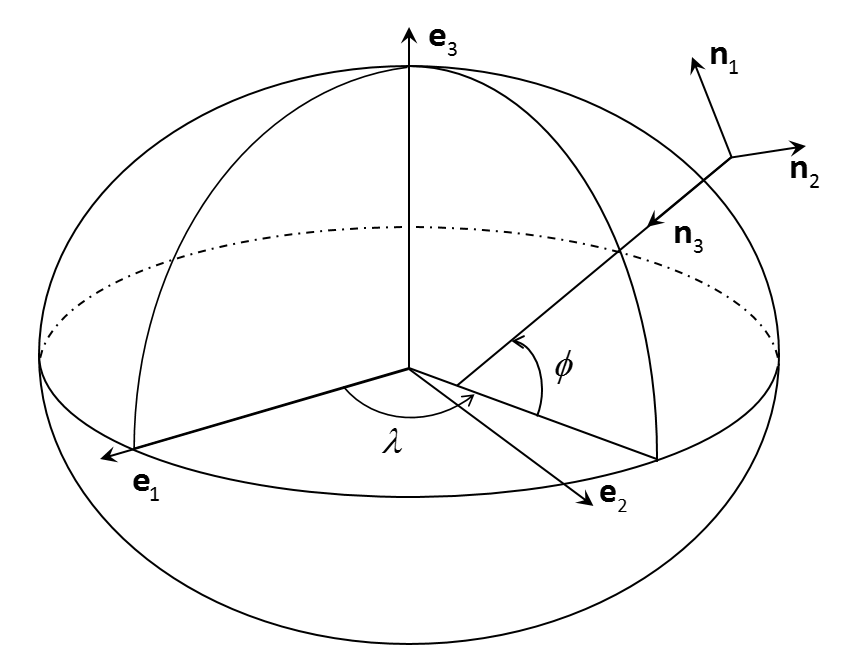
Fig. 2: n-frame
Navigation equations
Navigation equations are the first order ordinary differential equations that describe motion of a point mass in the neighborhood of Earth.
ECEF mechanizaton
\begin{eqnarray} \label{eq:ECEFnavEq} \dot{\mathbf{x}}_e & = & \mathbf{v}_e \\ \nonumber \dot{\mathbf{v}}_e & = & \mathbf{R}_{eb}(\breve{\mathbf{q}}_{eb}) \mathbf{f}_b + \mathbf{g}_e(\mathbf{x}_e) - 2\pmb{\omega}_{ie} \times \mathbf{v}_e \\ \nonumber \dot{\breve{\mathbf{q}}}_{eb} & = & \frac{1}{2} \left( \breve{\mathbf{q}}_{eb} \ast \breve{\pmb{\omega}}_{ib} - \breve{\pmb{\omega}}_{ie} \ast \breve{\mathbf{q}}_{eb} \right) \end{eqnarray}
Herein
- \( \mathbf{x}_e \) is the vector of the vehicle's cartesian coordinates in the ECEF frame;
- \( \mathbf{v}_e \) is the vector of the vehicle's velocity relative to the ECEF frame;
- \( \mathbf{R}_{eb} \) is the rotation matrix that defines the transformation from the b- to the e-frame;
- \( \mathbf{f}_b \) is the vector of specific force;
- \( \mathbf{g}_e \) is the Earth's gravity vector in the e-frame;
- \( \pmb{\omega}_{ie} = \begin{pmatrix} 0 & 0 & \omega_{ie} \end{pmatrix}^{\mathrm{T}} \) is the vector of the Earth's rotation rate;
- \( \pmb{\omega}_{ib} \) is the rate of rotation of the b-frame relative to the i-frame;
- \( \breve{\mathbf{q}}_{eb} \) is the rotation quaternion that defines the transformation from the b- to the e-frame;
- \( \breve{\pmb{\omega}}_{ib} \) and \( \breve{\pmb{\omega}}_{ie} \) are qaternions, whose scalar parts are equal to zero and whose vector parts are equal to \( \pmb{\omega}_{ib} \) and \( \pmb{\omega}_{ie} \), respectively.
NED mechanization
\begin{eqnarray} \label{eq:NEDnavEq} \dot{\pmb{\lambda}} & = & \mathbf{D}^{-1}(\pmb{\lambda})\mathbf{v}_n \\ \nonumber \dot{\mathbf{v}}_n & = & \mathbf{R}_{nb}(\breve{\mathbf{q}}_{nb}) \mathbf{f}_b + \mathbf{g}_n(\pmb{\lambda}) - \left( 2\mathbf{R}^{\mathrm{T}}_{en} \pmb{\omega}_{ie} + \pmb{\omega}_{en}(\pmb{\lambda},\mathbf{v}_n) \right) \times \mathbf{v}_n \\ \nonumber \dot{\breve{\mathbf{q}}}_{nb} & = & \frac{1}{2} \left( \breve{\mathbf{q}}_{nb} \ast \breve{\pmb{\omega}}_{ib} - \breve{\pmb{\omega}}_{in} \ast \breve{\mathbf{q}}_{nb} \right) \\ \nonumber \mathbf{D}(\pmb{\lambda}) & = & \begin{pmatrix} M(\phi)+h & 0 & 0 \\ 0 & (N(\phi) + h)\cos\phi & 0 \\ 0 & 0 & -1\end{pmatrix} \end{eqnarray}
Herein
- \( \pmb{\lambda} = \begin{pmatrix} \phi & \lambda & h\end{pmatrix}^{\mathrm{T}} \) is a vector composed of latitude, longitude, and height, respectively;
- \( \mathbf{v}_n = \begin{pmatrix} v_n & v_e & v_d \end{pmatrix}^{\mathrm{T}}= \mathbf{R}^{\mathrm{T}}_{en} \mathbf{v}_e \);
- \( \mathbf{R}_{en} \) is the rotation matrix that defines the transformation from the n- to the e-frame;
- \( \mathbf{R}_{nb} \) is the rotation matrix that defines the transformation from the b- to the n-frame;
- \( \mathbf{f}_b \) is the vector of specific force;
- \( \mathbf{g}_n \) is the Earth's gravity vector in the n-frame;
- \( \pmb{\omega}_{ie} = \begin{pmatrix} 0 & 0 & \omega_{ie} \end{pmatrix}^{\mathrm{T}} \) is the vector of the Earth's rotation rate;
- \( \pmb{\omega}_{en} \) is the rate of the n-frame relative to the e-frame, commonly known as the transport rate;
- \( \breve{\mathbf{q}}_{nb} \) is the rotation quaternion that defines the transformation from the b- to the n-frame;
- \( \pmb{\omega}_{ib} \) is the rate of rotation of the b-frame relative to the i-frame;
- \( \pmb{\omega}_{in} \) is the rate of rotation of the n-frame relative to the i-frame;
- \( \breve{\pmb{\omega}}_{ib} \) and \( \breve{\pmb{\omega}}_{in} \) are qaternions, whose scalar parts are equal to zero and whose vector parts are equal to \( \pmb{\omega}_{ie} \) and \( \pmb{\omega}_{in} \), respectively;
- \( M(\phi) \) and \( N(\phi) \) are the Earth's meridian and normal curvature radii.
Note that \begin{eqnarray*} \mathbf{R}^{\mathrm{T}}_{en}\pmb{\omega}_{ie} & = & \begin{pmatrix} \omega_{ie}\cos\phi & 0 & -\omega_{ie}\sin\phi \end{pmatrix}^{\mathrm{T}}, \\ \pmb{\omega}_{en} & = & \begin{pmatrix} \frac{v_e}{N(\phi) + h} & -\frac{v_n}{M(\phi) + h} & -\frac{v_e \tan\phi}{N(\phi) + h} \end{pmatrix}^{\mathrm{T}}, \\ \pmb{\omega}_{in} & = & \mathbf{R}^{\mathrm{T}}_{en}\pmb{\omega}_{ie} + \pmb{\omega}_{en}. \end{eqnarray*}
The Earth's normal and meridian curvature radii are given by $$ N(\phi) = \frac{a}{\sqrt{1 - e^2 \sin^2 \phi}}, \; M(\phi) = \frac{a(1- e^2)}{(1 - e^2 \sin^2 \phi)^{3/2}}, $$ where \( a \) and \( e \) are the semi-major axis and the eccentricity of the WGS84 ellipsoid of revolution.
Numerical integration of the navigation equations
Nonintegrating IMU
If IMU provides measurements of specific force and angular rate, the navigation equations (\ref{eq:ECEFnavEq}) and (\ref{eq:NEDnavEq}) can be integrated using classical numerical methods for solving ordinary differential equations, for example, the Euler method, or Runge-Kutta methods.
Integrating IMU
In case IMU outputs integrated measurements, i. e. velocity and angular increments, the navigation equations cannot be straightforwardly integrated. In this situation there are two alternative ways to proceed with solving them.
The first approach is called Conversion-Integration-Extrapolation (CIE). It supposes performing first a highly accurate conversion of the velocity and angular increments to the specific force and angular rate. Then the converted measurements may be used for numerical integration of the navigation equations by means of the conventional numerical methods. Finally, the obtained navigation solution needs to be extrapolated to the current time. To learn more about the CIE approach the reader can refer to [1].
The second approach consists in employing a very special numerical methods to integrate the navigation equations directly given the measurements of the velocity and angular increments. Below a method proposed in [1] is recapitulated.
\begin{eqnarray} \label{eq:SingleFreqAlgo} \mathbf{x}_e (t+\Delta t) & = & \mathbf{x}_e (t) + \mathbf{v}_e (t) \Delta t + \dot{\mathbf{v}}_e (t) \frac{\Delta t^2}{2!} + \ddot{\mathbf{v}}_e (t) \frac{\Delta t^3}{3!} \\ \nonumber \mathbf{v}_e (t+\Delta t) & = & \mathbf{v}_e (t) + \dot{\mathbf{v}}_e (t) \Delta t + \ddot{\mathbf{v}}_e \frac{\Delta t^2}{2!} \\ \nonumber \breve{\mathbf{q}}_{eb} (t+\Delta t) & = & \breve{\mathbf{p}}^{-1}_e \ast \breve{\mathbf{q}}_{eb} (t) \ast \breve{\mathbf{p}}_b \end{eqnarray}
Herein
\begin{eqnarray} \label{eq:SingleFreqAlgo1} \dot{\mathbf{v}}_e (t) & = & \mathbf{R}(\breve{\mathbf{q}}_{eb} (t)) \frac{\Delta \mathbf{v}^+_b + \Delta \mathbf{v}^-_b}{2 \Delta t} + \mathbf{g}_e(\mathbf{x}_e(t)) - 2 \pmb{\omega}_{ie} \times \mathbf{v}_e (t) \\ \nonumber \ddot{\mathbf{v}}_e (t) & = & \mathbf{R}(\breve{\mathbf{q}}_{eb} (t)) \left( \pmb{\omega}_{eb}(t) \times \frac{\Delta \mathbf{v}^+_b + \Delta \mathbf{v}^-_b}{2 \Delta t} + \frac{\Delta \mathbf{v}^+_b - \Delta \mathbf{v}^-_b}{\Delta t^2} \right) + \frac{\partial \mathbf{g}_e(\mathbf{x}_e(t))}{\partial \mathbf{x}^\mathrm{T}_e} \mathbf{v}_e(t) - \pmb{\omega}_{ie} \times \dot{\mathbf{v}}_e (t) \\ \nonumber \pmb{\omega}_{eb}(t) & = & \frac{1}{2 \Delta t} \left( \Delta \pmb{\theta}^+_{ib} + \Delta \pmb{\theta}^-_{ib} \right) - \mathbf{R}^\mathrm{T} (\breve{\mathbf{q}}_{eb} (t)) \pmb{\omega}_{ie} \\ \nonumber \breve{\mathbf{p}}_e & = & \left( \cos \left( \omega_{ie} \frac{\Delta t}{2} \right), \; \sin \left( \omega_{ie} \frac{\Delta t}{2} \right) \frac{\pmb{\omega}_{ie}}{\omega_{ie}} \right) \\ \nonumber \breve{\mathbf{p}}_b & = & \left( 1 - \frac{1}{8} || \Delta \pmb{\theta}^+_{ib}||^2, \; \frac{1}{2} \left( 1 - \frac{1}{24}|| \Delta \pmb{\theta}^+_{ib}||^2 \right) \Delta \pmb{\theta}^+_{ib} - \frac{1}{24} \Delta \pmb{\theta}^+_{ib} \times \Delta \pmb{\theta}^-_{ib} \right) \end{eqnarray}
The integrating IMU measurements are given by
\begin{eqnarray} \label{eq:IntIMUmeasDef} \Delta \pmb{\theta}^+_{ib} & = & \int^{t+\Delta t}_t \pmb{\omega}_{ib}(\tau) d \tau \\ \nonumber \Delta \pmb{\theta}^-_{ib} & = & \int^t_{t-\Delta t} \pmb{\omega}_{ib}(\tau) d \tau \\ \nonumber \Delta \mathbf{v}^+_b & = & \int^{t+\Delta t}_t \mathbf{f}_b (\tau) d \tau \\ \nonumber \Delta \mathbf{v}^-_b & = & \int^t_{t-\Delta t} \mathbf{f}_b (\tau) d \tau \end{eqnarray}
Further reading on integrating IMU algorithms can be found in [2].
[2] Savage, P.G., Strapdown Analytics, Vol. 1, Strapdown Associates, Inc., Mapl Plain, Minnessota, 1997.
INS initial alignment
Orientation of a vehicle relative to the NED frame can be determined by means of inertial sensors provided that the vehicle ramains stationary, i. e. does not move. The procedure is usually called levelling, or coarse alignment. At rest
\begin{equation*} \label{eq:InsAlignment1} \mathbf{R}_{nb} \cdot \mathbf{f}_b \approx \mathbf{g}_n \approx - \begin{pmatrix} 0 & 0 & || \mathbf{f}_b||\end{pmatrix}^\mathrm{T} \end{equation*}
Consequently,
\begin{eqnarray*} \label{eqInsAlignment2} f_x & = & || \mathbf{f}_b|| \sin \vartheta \\ \nonumber f_y & = & -|| \mathbf{f}_b|| \sin \varphi \cos \vartheta \\ \nonumber f_z & = & -|| \mathbf{f}_b|| \cos \varphi \cos \vartheta \end{eqnarray*}
Finally, the vehicle's roll and pitch angles, \( \varphi \) and \( \vartheta \), respectively, can be determined as
\begin{eqnarray*} \label{eq:InsAlignment3} \varphi & = & \mathrm{atan2} \left( \frac{-f_y}{-f_z} \right), \; \in [-\pi, \pi) \\ \nonumber \vartheta & = & \arcsin \left( \frac{f_x}{|| \mathbf{f}_b||} \right), \; \in [-\pi/2, \pi/2] \end{eqnarray*}
Determination of the heading angle \( \psi \) requires measurements of the gyroscopes and therefore is conventionally called gyrocompassing. A vehicle that is at rest on the Earth's surface is anyway turning, because the Earth itself is rotating. Since the gyroscopes measure the rate relative to some inertial reference frame,
\begin{equation*} \label{eq:Gyrocompassing1} \mathbf{R}_{nb} \cdot \pmb{\omega}_{ib} = \pmb{\omega}_{ie}^n \end{equation*}
By definition of Euler angles (aerospace sequence)
$$\mathbf{R}_{nb} = \mathbf{R}_3(\psi)\mathbf{R}_2(\vartheta)\mathbf{R}_1(\varphi)$$
Denote \( \pmb{\omega}_{ib}^h = \mathbf{R}_2(\vartheta)\mathbf{R}_1(\varphi) \cdot \pmb{\omega}_{ib} \). Then
$$\tan\psi = \frac{-\omega_{iby}^h}{\omega_{ibx}^h}$$
Finally, the vehicle's heading \( \psi \) can be computed as
\begin{equation*} \label{eq:Gyrocompassing2} \psi = \mathrm{atan2} \left( \frac{-\omega_{iby}^h}{\omega_{ibx}^h} \right) = \mathrm{atan2} \left( \frac{-\omega_{iby}\cos\varphi + \omega_{ibz}\sin\varphi }{\omega_{ibx}\cos\vartheta + \omega_{iby}\sin\varphi\sin\vartheta + \omega_{ibz}\cos\varphi\sin\vartheta } \right) , \: \in [-\pi, \pi). \end{equation*}
Advanced topics
- IMU error models
- Inertial meassurement unit calibration and testing
- Generating IMU data for simulation
- Platform inertial navigation systems
- Wander azimuth
To learn more about the advanced topics, please contact us!
Recommended literature
- Titterton, D.H., Weston, J. L., Strapdown Inertial Navigation Technology, Lavenham Press Ltd., UK, 1997.
- Farrell, J.A., Aided Navigation, GPS with High Rate Sensors, McGraw-Hill, USA, 2008.
- Groves, P.D., Principles of GNSS, Inertial, and Multisensor Integrated Navigation Systems, 2 ed, Artech House, Boston, 2013.